src.timed_net package

Summary

This simulations implements a temporal-aware PT net by attaching time information to the PT net tokens. It simulates a supply chain depending on two component producers and an assembler.

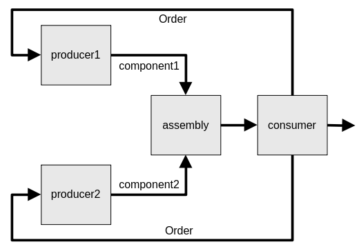
In the diagram,

• producer1 builds component1 in a time interval approximated by a normal distribution \(\mathcal{N}(\mu_1, \sigma_1)\) with the mean \(\mu_1\) and standard deviation \(\sigma_1\) seconds.

• Similarly producer builds component2 in a time interval of \(\mathcal{N}(\mu_2, \sigma_2)\)

• The components are assembled and served to the consumer.

• Lastly, the consumer places a new order to the producers.

The picture below is the auto-generated PT net diagram by SoyutNet.

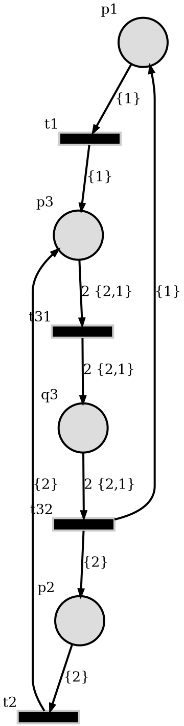
• p1 and t1 define the producer1.

• p2 and t2 define the producer2.

• t31 is the assembler.

• p3 is the consumer.

• The component1 and 2 are labeled by {1} and {2}.

System description

SoyutNet tokens are represented by a tuple of integers.

token: tuple[int, int] = (label, id)

Time information is embedded into the second item (id) of token. Simulation starts with an initial token at the producers

• produer1 has (PRODUCER1_LABEL, T0)

• produer2 has (PRODUCER2_LABEL, T0)

where T0 = 0 (secs) initially. Each producer adds a random integer distributed by \(\mathcal{N}(\mu_i, \sigma_i)\), \(i \in {1,2}\) at a (TimedTransition) instance then sends to their output arcs.

    class TimedTransition(soyutnet.Transition):
        def __init__(self, name, rng_params, *args, **kwargs):
            super().__init__(name=name, net=net, *args, **kwargs)
            self._rng_params = rng_params

        def _delay(self):
            return round(random.gauss(*self._rng_params))

        async def _process_tokens(self):
            for label in self._tokens:
                ids = self._tokens[label]
                self._tokens[label] = list(map(lambda x: x + self._delay(), ids))
                """Add producer delay"""

            return await super()._process_tokens()

The assembler receives tokens, redirects to the consumer. The total duration of this process is the maximum of the delay introduced by producers.

    class CombinerTransition(soyutnet.Transition):
        def __init__(self, *args, **kwargs):
            super().__init__(net=net, *args, **kwargs)
            self.arrival_time = []

        async def _process_tokens(self):
            max_id = 0
            arrivals = [0, 0]
            for label in self._tokens:
                ids = self._tokens[label]
                arrivals[label - 1] = max(ids)
                if ids:
                    max_id = max(max_id, arrivals[label - 1])
            for label in self._tokens:
                self._tokens[label] = [max_id] * len(self._tokens[label])
                """Total delay is the max of two branches"""

            self.arrival_time.append(arrivals)

            return await super()._process_tokens()

The consumer places an other order to the producers after receiving the token. At each cycle, the token IDs are incremented.

\[(label, t) \rightarrow (label, t+\Delta t)\]

The tokens are counted by the consumer and the timings are saved.

    production_time = TimeInstants()
    Ti = lambda k: production_time[k - 1]
    controller = Controller(production_time=production_time)
    converged = asyncio.Condition()

    async def stock_counter(tr):
        nonlocal production_time, converged
        t = None
        for label in tr._tokens:
            ids = tr._tokens[label]
            if not ids:
                continue
            for id in ids:
                if t is None:
                    t = id
                    production_time.append(t)
                else:
                    assert t == id

        dT = Ti(0) - Ti(-1)
        controller.measure(dT)
        u = controller.advance()
        """
        Measured production time and generated the amount of new order delays ``u``.
        u = (dt1, dt2) means that new order to producer1 and 2 will be placed after
        dt1 and dt2 seconds.
        """
        if controller.is_done():
            """If simulation is done inform the canceller."""
            async with converged:
                converged.notify_all()

        for i in range(2):
            """Postpone orders."""
            label = i + 1
            assert len(tr._tokens[label]) == 1
            tr._tokens[label][0] += u[i]

        return True

The whole implementation can be found at https://github.com/dmrokan/soyutnet-simulations/blob/main/src/timed_net/main.py

Joint probability distribution

The total duration of the described process is distributed according to

\[\begin{split}X &= \max{(X_1, X_2)} \\ X_i &\sim \mathcal{N}(\mu_i, \sigma_i) \Rightarrow E[X_i] = \mu_i, ~Var[X_i] = \sigma_i^2\end{split}\]

The mean and variance of \(X\) is given as

\[\begin{split}E[X] & = \mu_1 \Phi(\alpha) + \mu_2 \Phi(-\alpha) + \theta \phi(\alpha) \\ E[X^2] &= (\sigma_1^2+\mu_1^2) \Phi(\alpha) + (\sigma_2^2+\mu_2^2) \Phi(-\alpha) + (\mu_1 + \mu_2) \theta \phi(\alpha) \\ Var[X] &= E[X^2] - E[X]^2 \\ \theta &= \sqrt{\sigma_1^2+\sigma_2^2} \\ \alpha &= \frac{\mu_1-\mu_2}{\theta}\end{split}\]

where \(\Phi\) and \(\phi\) are the CDF and PDF of normal random distribution [nadarajah2008].

def pdf(x, mean=0, std=1):
    """phi"""
    var = std**2
    a = 2 * math.pi * var
    a = 1 / (a**0.5)
    return a * math.exp(-((x - mean) ** 2) / (2 * var))


def cdf(x, mean=0, std=1):
    """Phi"""
    a = 2**0.5
    return 0.5 * (1 + math.erf((x - mean) / (std * a)))

Real-time moment estimation

The moments \(E[X], E[X^2]\) and variance \(Var[X]\) can be estimated by dynamic averaging of observed random variable \(x_n\).

\[\begin{split}E[x_n] &= \mu \\ Var[x_n] &= E[x_n^2] - \mu^2 = \sigma^2\end{split}\]

For this purpose, a special list class NormalSamples is implemented.

    relative_error = lambda a, b, c=1 / (2**BIT_WIDTH - 1): abs((a - b) / (b + c))

    class NormalSamples(UserList):
        def __init__(
            self,
            *args,
            eps=1e-2,
            convergence_condition=10,
            rng_params=None,
            validate_conv=False,
        ):
            super().__init__(*args)
            self._eps = eps
            self._moments = None
            self._variance = Qp.tuple((0, eps, 0.0))
            self._cc = convergence_condition
            self._rng_params = None
            if rng_params is not None:
                self.set_rng_params(rng_params)
            self._max_size = 600 * 1024 * 1024
            self._initialize_moments()
            self._iter = 0
            self._validate_conv = validate_conv
            if validate_conv:
                self._last_n_dmu = Qp.list([0] * self._cc)
                self._last_n_dvar = Qp.list([0] * self._cc)

As products arrive, the difference between the ordering time and arrival time is calculated. When this delta time is appended to the NormalSamples, it automatically updates moments and variance.

        def _update_moment(self, moment, val):
            moment = Qp.tuple(moment)
            if abs(val) < 1e-2 * self._eps:
                """Ignore very small numbers in statistics"""
                return moment
            l = len(self)
            mu, eps, eps0 = moment
            if l % self._cc == 0:
                eps0 = 0.0
            mu_prev = mu
            mu = (mu * l + val) / (l + 1)
            dmu = relative_error(mu_prev, mu)
            eps = (eps * l + dmu) / (l + 1)
            eps0 = max(eps0, eps)
            assert isinstance(mu, Qp)
            assert isinstance(eps, Qp)
            assert isinstance(eps0, Qp)
            """
            Save the max of last self._cc samples which
            will be used for deciding convergence later.
            """

            return (mu, eps, eps0)

If last N samples are very close to each other distrbution, the NormalSamples instance informs about convergence.

• mu is the estimate of moment calculated by dynamic averaging.

• eps the average change in current and previous mu.

• eps0 is the max of last self._cc number of eps values which is used to determine convergence.

Estimate producer delays

The problem is developing an algorithm to estimate the producer delays separately by using the difference between the time a new order is placed and the time when the product is received.

System model

A simple model of the producer/consumer flow can be

\[\begin{split}x_1[n+1] &= w_1[n] + u_1[n] \\ x_2[n+1] &= w_2[n] + u_2[n] \\ x[n+1] &= \max\left\{x_1[n], x_2[n]\right\} \\ y[n] &= x[n]\end{split}\]

• \(n\) is the product counter starting from zero.

• \(x_i\) is the production time of component_i.

• \(w_i\) is a Gaussian random variable, \(E[w_i] = \mu_i, Var[w_i] = \sigma_i^2\).

• \(y = x\) is the total production observed by the consumer, \(E[y] = \mu, Var[y] = \sigma^2\).

• \(u_i (sec)\) denotes postponing the orders by the consumer. It is assumed that the consumer can schedule orders for later instead of placing them immediately.

• The units are seconds.

State machine observer/controller scheme

The observer/controller scheme runs a few tests on the producer/consumer flow. The order of tests are implemented as a state machine with the states below

    class State(Enum):
        OBSERVE_JOINT_DIST = auto()
        TEST_PRODUCER1 = auto()
        TEST_PRODUCER2 = auto()
        ESTIMATE_DELAYS = auto()
        DONE = auto()

• OBSERVE_JOINT_DIST: Estimate joint mean (\(\mu\)) and variance (\(\sigma\)).

• TEST_PRODUCER1: Find out producer1’s response by postponing orders.

• TEST_PRODUCER2: Find out producer2’s response by postponing orders.

• ESTIMATE_DELAYS: Calculate the difference between \(\mu_1\) and \(\mu_2\) approximately.

• DONE: Exit simulation.

The state machine is implemented as below.

        def advance(self):
            """Iterate the controller"""
            match self._state[0]:  # Check current state
                case State.OBSERVE_JOINT_DIST:  # Initial state
                    """1. Validate that total production time is as expected."""
                    mu, std, conv = self.found()
                    assert isinstance(mu, int)
                    assert isinstance(std, int)
                    if conv:  # Check convergence
                        self._observed.append(self._u + (mu, std))
                        match self._state[-1]:  # Check previous state
                            case State.OBSERVE_JOINT_DIST:
                                self._change_state(State.TEST_PRODUCER1)
                            case State.TEST_PRODUCER1:
                                self._change_state(State.TEST_PRODUCER2)
                            case State.TEST_PRODUCER2:
                                self._change_state(State.ESTIMATE_DELAYS)
                            case State.ESTIMATE_DELAYS:
                                self._change_state(State.DONE)
                case State.TEST_PRODUCER1:
                    """2. Postpone ordering from producer1"""
                    self._u = (self._mu0, 0)
                    self._update_rng_params(tuple(self._u))
                    self._change_state(State.OBSERVE_JOINT_DIST)
                case State.TEST_PRODUCER2:
                    """3. Postpone ordering from producer2"""
                    self._u = (0, self._mu0)
                    self._update_rng_params(tuple(self._u))
                    self._change_state(State.OBSERVE_JOINT_DIST)
                case State.ESTIMATE_DELAYS:
                    """4. Estimate the slow producer"""
                    test1 = self._observed[1]
                    test2 = self._observed[2]
                    dt = test1[2] - test2[2]
                    index = int(dt > 0)
                    dt = abs(dt)
                    self._slow_producer = (index + 1, dt)
                    self._u = (0, 0)
                    self._update_rng_params(tuple(self._u))
                    self._change_state(State.OBSERVE_JOINT_DIST)

            return tuple(map(int, self._u))

1. Set \(u_1[n] = u_2[n] = 0\) for all n,

2. OBSERVE_JOINT_DIST: Estimate the reference \((\mu_0, \sigma_0)\) and record.

3. TEST_PRODUCER1: Set \(u_1[n] = \mu_0, u_2[n] = 0\) for all n.

4. OBSERVE_JOINT_DIST: Estimate \((\mu_1, \sigma_1)\) and record.

5. TEST_PRODUCER2: Set \(u_1[n] = 0, u_2[n] = \mu_0\) for all n.

6. OBSERVE_JOINT_DIST: Estimate \((\mu_2, \sigma_2)\) and record.

7. ESTIMATE_DELAYS: The difference between the production time of producers is \(dt = |\mu_1 - \mu_2|\) and the index of slow producer is int(dt > 0) + 1.

8. DONE: Exit.

Integer arithmetic implementation

In this simulation, all calculations are done on Python’s Fraction instances instead of float s. This simulation implements a new class called Qp to ensure all basic math operations returns a Fraction.

A Fraction can be instantiated by an int, float, str and it converts the input to a tuple of (numerator, denominator) of type tuple[int, uint]. Also, a limit to the denominator can be set. For example:

>>> Fraction(-0.3).limit_denominator(10)
Fraction(-3, 10)
>>> Fraction(0.3).limit_denominator(2)
Fraction(1, 2)
>>> Fraction(0.3).limit_denominator(1)
Fraction(0, 1)

In the example, Fraction(0, 1) and Fraction(-3, 10) are equivalent to \(0/1\) and \(-3/10\). As the denominator limit increases, the precision of calculations increases. Because, the numbers less than one can still be represented in the calculations.

    class Qp:
        def __init__(self, num=0, max_den=(2**BIT_WIDTH - 1)):
            self._max_den = max_den
            if isinstance(num, Qp):
                num = num.num
            self.num = self._new_num(num)

        def _new_num(self, num):
            return Fraction(num).limit_denominator(self._max_den)

        @staticmethod
        def tuple(iterable):
            return tuple(map(Qp, iterable))

        @staticmethod
        def list(iterable):
            return list(map(Qp, iterable))

        def int_op(op, swap=False):
            def inner(func):
                def wrapped(self, *args):
                    a, b = self, Qp(args[0])
                    if swap:
                        a, b = b, a
                    return Qp(op(a.num, b.num))

                return wrapped

            return inner

        # fmt: off
        @int_op(operator.mul)
        def __mul__(self, other): ...
        @int_op(operator.truediv)
        def __truediv__(self, other): ...
        @int_op(operator.add)
        def __add__(self, other): ...
        @int_op(operator.sub)
        def __sub__(self, other): ...
        @int_op(operator.pow)
        def __pow__(self, other): ...
        @int_op(operator.gt)
        def __gt__(self, other): ...
        @int_op(operator.lt)
        def __lt__(self, other): ...

        @int_op(operator.mul, True)
        def __rmul__(self, other): ...
        @int_op(operator.truediv, True)
        def __rtruediv__(self, other): ...
        @int_op(operator.add, True)
        def __radd__(self, other): ...
        @int_op(operator.sub, True)
        def __rsub__(self, other): ...
        @int_op(operator.pow, True)
        def __rpow__(self, other): ...
        # fmt: on

        def __str__(self):
            return str(self.num)

        def __float__(self):
            return float(self.num)

        def __int__(self):
            return int(self.num)

        def __abs__(self):
            return Qp(abs(self.num))

        def is_zero(self, eps=1e-2):
            eps = max(eps, 1 / self._max_den)
            return abs(self) < Qp(eps)

By using this reference implementation, it can be translated to work on an MCU platform. However, it will require limiting the magnitude of numerator together with the denominator. Because, the integer size is unlimited in Python.

Results

The simulation is run for several different \(\mu_i\) and \(\sigma_i\) as defined below in __main__.py

RNG_PARAMS = [
    #mu_1,   sigma_1,   mu_2,    sigma_2 (minutes)
    (100,    5,         100,     5),
    (100,    25,        100,     25),
    (100,    5,         50,      5),
    (50,     5,         100,     25),
    (100,    5,         20,      5),
    (20,     5,         100,     25),
]

The table below shows the joint probability distribution characteristics.

• mu0 is \(E[X]\) in the equation above.

• std0 is \(\sqrt{Var[X]}\) in the equation above.

• mu is obtained by calculating the mean of the difference of saved timings.

• std is obtained by calculating the standard deviation of the difference of saved timings.

• The values are in seconds.

Table 1: Average and actual values.

mu	mu0	std	std0
6232	6169	181	247
6942	6846	1241	1238
5943	6000	229	299
5806	6014	1269	1467
5817	6000	248	300
5977	6000	1582	1498
5987	6169	199	247
6504	6846	950	1238
5933	6000	309	299
6199	6014	1651	1467
6045	6000	378	300
6093	6000	1355	1498

The next table shows estimation results.

• weak = 1 means that only mean values are used to determine convergence.

• eps is the relative error tolerance to determine convergence.

• iter is the final value of the product counter.

• mu, mu0 and Dmu are estimated, actual mean value and the relative error.

• std, std0 and Dstd are estimated, actual standard deviation and the relative error.

• slow is the estimated slow producer indices (‘*’ indicates wrong estimation).

• Dt, Dt0 and err are estimated, actual production delay differences and their relative error.

  e.g. slow = 1 and Dt = 1000 mean the producer1 is 1000 seconds slower than the producer2.

• The values are in seconds except weak, iter and slow, former are unitless.

Table 2: Observer estimations (when max rational number denominator is 1. Meaning, the mean and variance are calculated by using integer arithmetic).

weak	eps	iter	mu	mu0	Dmu	std	std0	Dstd	slow	Dt	Dt0	err
0	0.01	47	6231	6169	0.01	1	247	0.992	2*	1	0	0.99
0	0.01	47	6942	6846	0.014	1	1238	0.998	2*	293	0	1.0
0	0.01	47	5943	6000	0.009	1	299	0.993	2	3014	3000	0.0
0	0.01	47	5806	6014	0.035	1	1467	0.999	1	2910	3000	0.03
0	0.01	47	5819	6000	0.03	1	300	0.993	2	4744	4800	0.01
0	0.01	47	5978	6000	0.004	1	1498	0.999	1	4097	4800	0.17
1	0.01	47	6141	6169	0.005	1	247	0.992	2*	107	0	1.0
1	0.01	47	6182	6846	0.097	1	1238	0.998	2*	758	0	1.0
1	0.01	47	5895	6000	0.017	1	299	0.993	2	3122	3000	0.04
1	0.01	47	5440	6014	0.095	1	1467	0.999	1	3325	3000	0.1
1	0.01	47	5947	6000	0.009	1	300	0.993	2	4936	4800	0.03
1	0.01	47	6357	6000	0.059	1	1498	0.999	1	5175	4800	0.07
0	0.1	47	6151	6169	0.0	1	247	0.99	2*	126	0	1.0
0	0.1	47	7193	6846	0.05	1	1238	1.0	1	705	0	1.0
0	0.1	47	5902	6000	0.02	1	299	0.99	2	2968	3000	0.01
0	0.1	47	6136	6014	0.02	1	1467	1.0	1	2621	3000	0.14
0	0.1	47	5859	6000	0.02	1	300	0.99	2	4975	4800	0.04
0	0.1	47	5899	6000	0.02	1	1498	1.0	1	4414	4800	0.09
1	0.1	47	6179	6169	0.0	1	247	0.99	1	70	0	1.0
1	0.1	47	6982	6846	0.02	1	1238	1.0	2*	807	0	1.0
1	0.1	47	5871	6000	0.02	1	299	0.99	2	3115	3000	0.04
1	0.1	47	6381	6014	0.06	1	1467	1.0	1	3467	3000	0.13
1	0.1	47	5972	6000	0.0	1	300	0.99	2	4910	4800	0.02
1	0.1	47	6155	6000	0.03	1	1498	1.0	1	4761	4800	0.01

Table 3: Observer estimations (when max rational number denominator is 255).

weak	eps	iter	mu	mu0	Dmu	std	std0	Dstd	slow	Dt	Dt0	err
0	0.01	47	5987	6169	0.03	205	247	0.17	1	28	0	1.0
0	0.01	47	6504	6846	0.05	855	1238	0.309	2*	853	0	1.0
0	0.01	47	5933	6000	0.011	286	299	0.043	2	2838	3000	0.06
0	0.01	47	6199	6014	0.031	1506	1467	0.027	1	2963	3000	0.01
0	0.01	47	6045	6000	0.007	339	300	0.13	2	4722	4800	0.02
0	0.01	47	6093	6000	0.015	1227	1498	0.181	1	4565	4800	0.05
1	0.01	47	6271	6169	0.017	249	247	0.008	2*	89	0	1.0
1	0.01	47	7733	6846	0.13	1020	1238	0.176	1	319	0	1.0
1	0.01	47	5864	6000	0.023	359	299	0.201	2	3238	3000	0.07
1	0.01	47	6277	6014	0.044	1958	1467	0.335	1	3258	3000	0.08
1	0.01	47	5812	6000	0.031	315	300	0.05	2	4829	4800	0.01
1	0.01	47	5241	6000	0.126	1214	1498	0.19	1	4532	4800	0.06
0	0.1	47	6150	6169	0.0	171	247	0.31	1	114	0	1.0
0	0.1	47	6355	6846	0.07	1022	1238	0.17	1	730	0	1.0
0	0.1	47	5926	6000	0.01	147	299	0.51	2	2957	3000	0.01
0	0.1	47	5909	6014	0.02	1417	1467	0.03	1	3326	3000	0.1
0	0.1	47	5925	6000	0.01	277	300	0.08	2	4764	4800	0.01
0	0.1	47	6497	6000	0.08	1324	1498	0.12	1	5304	4800	0.1
1	0.1	47	6143	6169	0.0	202	247	0.18	2*	60	0	1.0
1	0.1	47	6682	6846	0.02	1019	1238	0.18	2*	1127	0	1.0
1	0.1	47	6146	6000	0.02	256	299	0.14	2	3006	3000	0.0
1	0.1	47	6199	6014	0.03	890	1467	0.39	1	2470	3000	0.21
1	0.1	47	5967	6000	0.01	276	300	0.08	2	4773	4800	0.01
1	0.1	47	5496	6000	0.08	1454	1498	0.03	1	4791	4800	0.0

Comments

• Table 1 shows that mean and variance is very close to the values obtained from the results of equations.

• Table 2 shows that estimator works correctly even if it operates on integers. But, it can not estimate the variance by using integer precision.

• Table 3 shows that estimator works correctly when fractional numbers are used. And, it can more or less estimate the variance.

  It is hard to estimate small differences between \(\mu_1\) and \(\mu_2\).

References

[nadarajah2008]

S. Nadarajah and S. Kotz, “Exact Distribution of the Max/Min of Two Gaussian Random Variables,” 2008

Reproduce

sudo apt install python3-venv graphviz
python3 -m venv venv
source venv/bin/activate

make build
make build=timed_net
make clean=timed_net
make run=timed_net
make results=timed_net
make graph=timed_net
make docs

Usage

Submodules

src.timed_net.main module

src.timed_net.main.USAGE()

Arguments:

-r <rng params>

mu1,std1,mu2,std2 (units are seconds)

Default: 300,60,600,180

-T <time (sec)>

total simulation time in seconds

Default: 2

-o <filename>

output file name to write results. If empty, prints to stdout.

-G

if provided, the script generates PT net graph and exits

-W

if provided, uses a weak comparion metric for convergence which highly increase simulation speed with the cost of degraded accuracy.

-C <strict|weak>

Controller type. ‘weak’ is equivalent to setting -W argument.

Default: strict

-e eps

Relative tolerance to determine convergence.

Default: 1e-2

-b denominator bit width (bw)

The denominator of Fraction used in calculations are limited to 2^(bw)-1

Example

python src/timed_net/main.py -r 100,10,200,25 -T 2

src.timed_net.results module

src.timed_net.results.cdf(x, mean=0, std=1)

Phi

src.timed_net.results.joint_mean(dist1, dist2)

src.timed_net.results.joint_variance(dist1, dist2)

src.timed_net.results.load_results()

src.timed_net.results.main(argv)

src.timed_net.results.pdf(x, mean=0, std=1)

phi

Module contents